How to Create Interactive Excel Pie Chart: 7 Steps

The pie chart is easy to be overwhelmed with data. This is easily solved if the user can select a specific item and the chart shows the pie slice for that item. You will learn how to create an interactive Excel pie chart in this article.

Here is a video overview of what we will achieve after reading through this.

 

Download Section

Interactive Pie Chart.xlsx

Interactive Excel Pie Chart: 2 Approaches

The first approach is combining formula and chart features to generate an interactive pie chart in Excel. The next approach is to make use of the pivot table feature.

Before everything else, let us look at our dataset. There are 3 columns that contain the list of items, their ingredient list, and the percentage of each ingredient. Our goal is to display the ingredient percentages for any selected items using a dynamic pie chart.

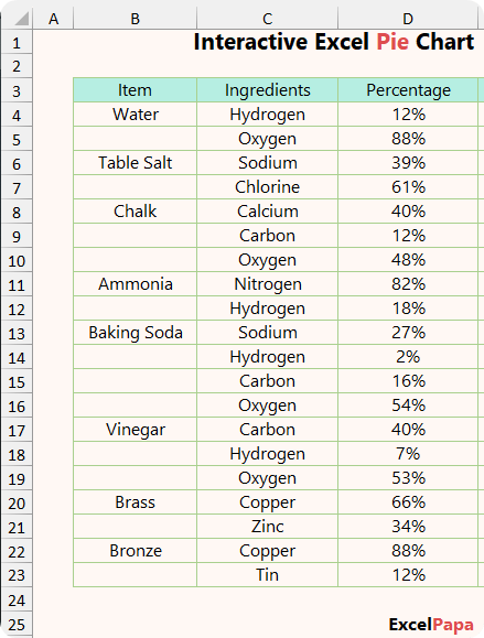
Let us investigate how to achieve this. Initially, using formulas and then utilizing the pivot table feature.

Using Formulas

If we look closely at the dataset, we will notice that the item column contains blank values for the same item. If we populate all the cells with values, then it will be easier to work. So, in the first step we will create a helper column to do so. Additionally, the values are converted into a table (Note: this is optional but it will make things more dynamic).

Then, we will find the unique item list. After that, a drop-down list is created, which will be used to change the item list. Following that, the associated ingredients will be returned. Then, using the item and ingredient list, a multiple criteria lookup formula will return the ingredient percentages.

Afterward, we create a pie chart from those values. Following that, the chart value, series values, and axis labels will then be dynamically updated to reflect the new values selected from the drop-down list. Finally, some chart formatting will take place to make it visually appealing to the audience.

Step I: Creating Helper Column

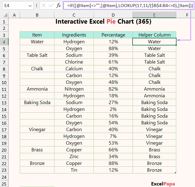
The dataset is converted into a table (filter button hidden). Use the formula to repeat the item names. Working with blank cells can be a nightmare, so we are doing this to type the related item list for the ingredients.

=IF([@Item]<>””,[@Item],LOOKUP(17,11/($B$4:B4<>0),[Item]))

[Understanding the Formula]

• @Item means the current item name from the current row and [Item] denotes the Item column.
• IF([@Item]<>””,[@Item]
  • This means if the item from a row is not blank, then it will return the value of the row.
• LOOKUP(17,11/($B$4:B4<>0)
  • Let us further break this down.
  • $B$4:B4<>0
    • $B$4 will be fixed for all formulas, but the next cell range, B4, will be changed to E5, then F5, and so on.
    • It is checking if the cell range is not blank (0 means blank cell).
    • Output will be a boolean value, either true or false.
  • 11/($B$4:B4<>0)
    • Dividing the boolean value by a number. You can take any number here instead of 11.
    • When false is divided by a number, then it will throw the #Div/0! error.
  • Finally, 17 is looked up in the formula in the LOOKUP(17,11/($B$4:B4<>0) part.
    • You can type any number more than 11.
    • The LOOKUP function looks for a value 17 in the formula, which will not be found. So, it gives the approximate match from the lookup vector. This will return the last non-blank cells from the floating cell reference.
  • The formula will therefore return the row value if the item is not blank and the last non-empty item name otherwise.

Step II: Finding Unique Items

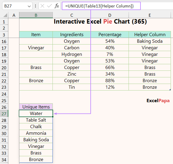
Now, we will find the unique item list from the dataset. To do so, insert this formula.

=UNIQUE(Table13[Helper Column])

If you are using an earlier version of Excel, then you can use the following formula to find the unique values.

=LOOKUP(17,11/((COUNTIF($B$27:B27,Table1[Item])=0)*(COUNTIF(Table1[Item],Table1[Item])=1)),Table1[Item])

[Understanding the Formula]

• This formula is used in the “sh” sheet. That is why Table1 is showing in the formula. Let us observe the formula part by part.
•  COUNTIF($B$27:B27,Table1[Item])=0
  • $B$27:B27 is a dynamic range and it expands as the formula goes to the next row.
  • This checks if the current value from Table1[Item] column is unique in the range.
• COUNTIF(Table1[Item],Table1[Item])=1
  • This makes sure the value in the Table1[Item] column is unique in the same column.
• The multiplication of the two formulas will be 1 if both are unique.
• Then, as previously mentioned, the Lookup function works.

Step III: Creating Drop-down List

In the third step, we will use the unique item list to create a drop-down list in Excel. This list will be the switch to control the interactive Excel pie chart.

• Firstly, select any cell.
• Secondly, from the Data tab, select Data Validation.
• Thirdly, select these in the respective fields.
  • Allow: List.
  • Source: B27:B34 (from step II).
• After that, press OK to complete this process.

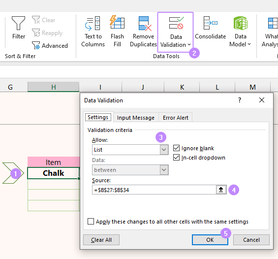
When you click on that cell, an arrow will appear, which you can use to change it to any item.

Step IV: Returning Ingredients

Now, we will return all ingredients for the selected item with the formula below. This formula filters the table when the value of the helper column matches the value of the drop-down list item.

=FILTER(Table13[Ingredients],Table13[Helper Column]=$H$8)

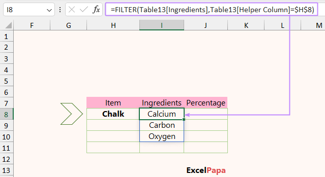
Alternatively, for earlier versions of Excel, use this formula instead.

=IFERROR(INDEX(Table1[Ingredients],SMALL(IF($H$8=Table1[Helper Column],ROW(Table1[Helper Column])-ROW($E$4)+1),ROW(1:1))),””)

[Understanding the Formula]

• IF($H$8=Table1[Helper Column],ROW(Table1[Helper Column])-ROW($E$4)+1)
  • It finds the relative row number if the item name is the same as the Table1[Helper] column.
• Then, using the current position and beginning with the first match, the SMALL function returns the smallest row number from the matches.
• After that, the row number from the SMALL function returns a value with the help of the INDEX function.
• Lastly, the IFERROR function is used to return a blank value if any error occurs.

Step V: Multiple Criteria Lookup

After that, we need the percentage of the item ingredients. For doing that, apply this formula.

=FILTER(Table13[Percentage], (Table13[Helper Column]=$H$8) * (ISNUMBER(MATCH(Table13[Ingredients], FILTER(Table13[Ingredients], Table13[Helper Column]=$H$8), 0))))

[Understanding the Formula]

• MATCH(Table13[Ingredients], FILTER(Table13[Ingredients], Table13[Helper Column]=$H$8), 0)
  • This portion checks if all the ingredients from the Table13[Ingredients] columns appear in the filtered list.
  • Then, the ISNUMBER function is used to convert the matched values to true and unmatched to false.
• Table13[Helper Column]=$H$8)
  • This checks if the value from the drop-down list matches value from the helper column.
• Then, this is multiplied with the previous formula. Both of them must be true to be incorporated into the formula.
• Lastly, the FILTER function filters and returns the percentage column.

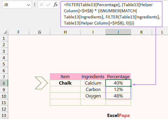
If the FILTER function is not available in your Excel, then use this formula instead.

=IFERROR(INDEX(Table1[Percentage],MATCH(1,(Table1[Helper Column]=$H$8)*(Table1[Ingredients]=I8),0)),””)

[Understanding the Formula]

• Table1[Helper Column]=$H$8
  • This checks if the value from the drop-down list matches with the value from the helper column.
• Table1[Ingredients]=I8
  • The first ingredient value is matched in the ingredients column.
• After that, these two are multiplied. When both of these matches then, it will return 1.
• Then, the MATCH function kicks in and calculate the row number of the first 1.
• Afterward, the INDEX function returns the percentage value for the row number.
• Lastly, the IFERROR function is used to handle any errors.

Step VI: Inserting Pie Chart

At first, we will insert the basic pie chart. Then, we will make the chart values and labels dynamic. This is done to remove the blank values from the chart.

• First of all, select the ingredients and percentage values that we got from steps IV & V.
• Then, from the Insert tab, select Pie or Doughnut chart.
• Afterward, select Pie from the 2-D pie section.

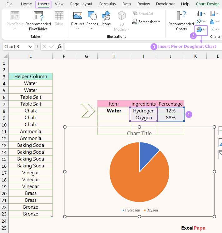
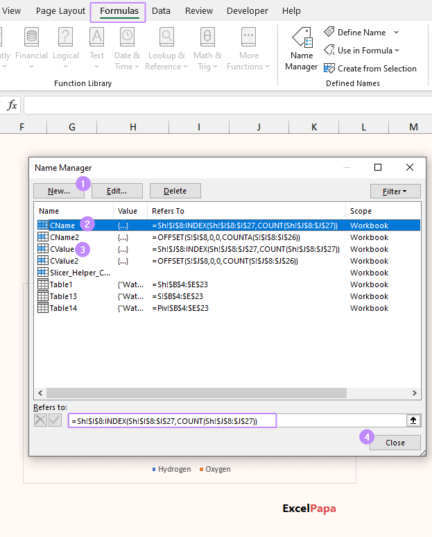
Then, we will use the Name Manager to make the pie chart values dynamic, which will make it interactive in Excel.

• From the Formulas tab, select Name Manager.
• Then, select New and input the following names to return the ingredient list.
  • Name: CName. You can type here any name you like.
  • Refers To: =Sh!$I$8:INDEX(Sh!$I$8:$I$27,COUNT(Sh!$J$8:$J$27)). This formula will return the last row for the selected items from the drop-down list. This formula is used in the ”Sh” sheet.
  • Alternatively, you can use =OFFSET(S!$I$8,0,0,COUNTA(S!$I$8:$I$26)) in the Refer To field to do the same. This formula is used in the “S” sheet.
• After that, use the formula to refer to the relevant percentage values of the selected item.
  • Name: CValue.
  • Refers To: =Sh!$J$8:INDEX(Sh!$J$8:$J$27,COUNT(Sh!$J$8:$J$27)).
  • An alternative formula =OFFSET(S!$J$8,0,0,COUNT(S!$J$8:$J$26)) is used in the CValue2 Name.
• Press Close to finish this process. We will use these custom names to make the pie chart interactive in Excel.

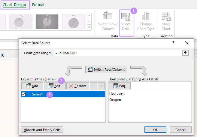
Select the pie chart and from the Chart Design tab, press Select Data and edit the Series1 data.

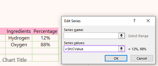
Then, input the custom name CValue in the value field. Here, “Sh!” denotes the “Sh” sheet and without this it will not work.

Similarly, use the other custom name for the axis label range. Then, press OK. It will make the chart dynamic.

After that, we will make the chart label change with the item too. Select the chart label and in the formula bar type =Sh!$H$8.

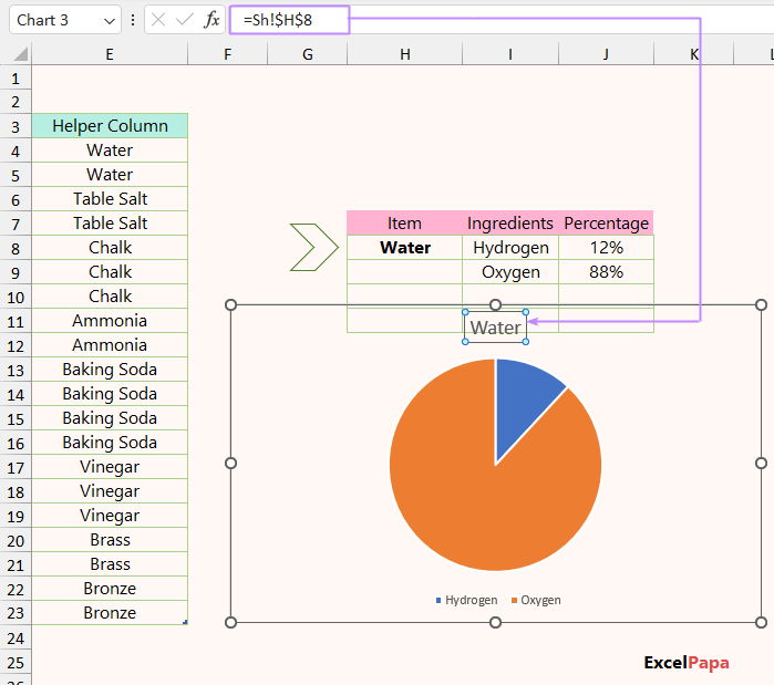
Step VII: Formatting

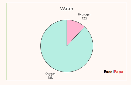
You can play with the shape outline, shape fill, and data label of the pie chart to make it look more appealing. Moreover, you can learn about various color theories to make any chart stand out. Below you can see a modified pie chart.

Now, let us see another way make the Excel interactive pie chart without using the name manager and complex formulas.

Using Pivot Table

You can also use the pivot table feature to create the data for the pie chart. You do not need to use formulas to find the unique values and their instances in this way. Does it look appealing? Yes! We will discuss this in brief. To do this,

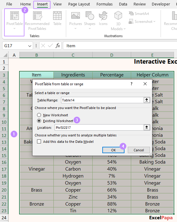
• At the beginning, select the data.
• Then, from the Insert tab, select PivotTable.
• After that, select the destination point and press OK.

• Afterward, drag the fields (table columns) to the following areas:
  • Helper Column and Ingredients into the Rows.
  • Ingredients into Value.
• Then, remove all subtotals and grand totals.
• Set the report layout to show in compact form.
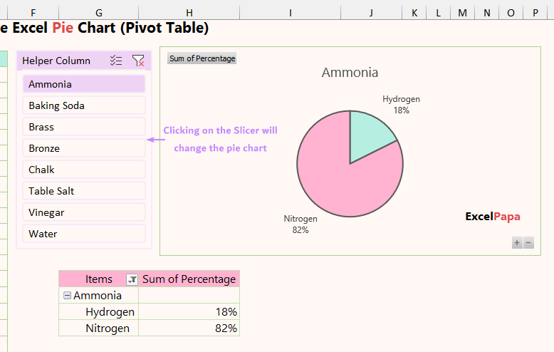
• After that, insert a slicer from the PivotTable Analyze tab. This slicer will be used to change the pie chart. Select the Helper Column in the dialog box that appears.
• Finally, modify the chart and slicer to finish this task.

Frequently Asked Questions (FAQ)

01. Where can I get a interactive pie chart template?

We have given the excel file in the article. You can modify this to accommodate your need. This is a freely downloadable xlsx file.

02. How to make pie chart in Excel with percentages?

You can just select your dataset and then use the Insert Pie Chart feature of excel to do so. Remember to convert your data to percentage first.

03. How to make an excel pie chart that look professional?

You need to use minimal styles on the pie chart. Remove unnecessary labels, gridlines, fills, and outlines. Moreover, use eye soothing custom colors in the pie chart to make it look like more professional.

04. How do I activate Pie Chart in Excel?

You can activate pie chart or any other charts in Excel by clicking on the chart itself. Additionally, the mouse pointer will change once you hover your mouse on the chart area.

Things to Remember

1. Always use the sheet name as prefix in the series value and axis label field.
2. Avoid using too much volatile functions (OFFSET, INDIRECT, etc.). As it may slow down your worksheet.
3. You may get a job interview where the Excel version may be old. So, learning bigger but more compatible formulas are key to ace in any kinds of interview or circumstances. So, keep an open mind to learn alternative formula for any task.

Epilogue

You can learn more about us here. We have used a lot of functions and formulas and other Excel features in this article. The formulas may be large but we try to explain them in simpler terms. Despite that, feel free to contact us if you face any difficulty understanding the Excel interactive pie chart.  Have a nice day, and thanks for reading. We wish you excel in your life!